Joint Distributions
Joint Distributions concerned with joint probability structure of two or more random variables defined on the same sample space.Joint distributions arise naturally in many applications.
• The joint probability distribution of the x, y, and z components of wind velocity can be experimentally measured in studies of atmospheric turbulence.
• The joint distribution of the values of various physiological variables in a population of patients is often of interest in medical studies.
• A model for the joint distribution of age and length in a population of fish can be used to estimate the age distribution from the length distribution. The age distribution is relevant to the setting of reasonable harvesting policies.
The joint behavior of two random variables, $X$ and $Y$, is determined by the cumulative distribution function
$F(x, y) = P(X ≤ x, Y ≤ y)$
regardless of whether $X$ and $Y$ are continuous or discrete. The cdf gives the probability that the point $(X, Y )$ belongs to a semi-infinite rectangle in the plane, as shown in Figure below. The probability that $ (X, Y )$ belongs to a given rectangle is, from Figure (b) is ,
$P(x1 < X ≤ x2, y1 < Y ≤ y2) = F(x2, y2) − F(x2, y1) − F(x1, y2) + F(x1, y1)$
The probability that $(X, Y )$ belongs to a set A, for a large enough class of sets for practical purposes, can be determined by taking limits of intersections and unions of rectangles. In general, if $X1, . . . , Xn$ are jointly distributed random variables, their joint cdf is
$F(x1, x2, . . . , xn) = P(X1 ≤ x1, X2 ≤ x2, . . . , Xn ≤ xn)$
Discrete Random Variables
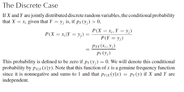
Suppose that $X$ and $Y$ are discrete random variables defined on the same sample space and that they take on values $x1, x2, . . . ,$ and $y1, y2, . . . $, respectively. Their joint frequency function, or joint probability mass function, $p(x, y)$, is
$ p(xi , yj ) = P(X = xi , Y = yj )$
A simple example will illustrate this concept. A fair coin is tossed three times; let $X$ denote the number of heads on the first toss and $Y$ the total number of heads. From the sample space, which is
$\omega = {hhh, hht, hth, htt, thh, tht, tth, ttt}$
Thus, for example, $p(0, 2) = P(X = 0, Y = 2) = 1/8$
Note that the probabilities in the preceding table sum to 1.
Suppose that we wish to find the frequency function of $Y$ from the joint frequency function. This is straightforward:
$p_Y (0) = P(Y = 0)$
$\quad = P(Y = 0, X = 0) + P(Y = 0, X = 1)$
$\quad = 1/8+ 0= 1/8$
$p_Y (1) = P(Y = 1)$
$\quad = P(Y = 1, X = 0) + P(Y = 1, X = 1)$$\quad = 3/8$
In general, to find the frequency function of $Y $, we simply sum down the appropriate column of the table. For this reason, $p_Y$ is called the marginal frequency function of $Y$ . Similarly, summing across the rows gives
$p_X (x) =\sum_i p(x,y_i)$
which is the marginal frequency function of $X$.
The case for several random variables is analogous. If $X1, . . . , Xm$ are discrete random variables defined on the same sample space, their joint frequency function is
$p(x1, . . . , xm) = P(X1 = x1, . . . , Xm = xm)$
Multinomial Distribution
The multinomial distribution, an important generalization of the binomial distribution, arises in the following way. Suppose that each of $n$ independent trials can result in one of $r$ types of outcomes and that on each trial the probabilities of the $r$ outcomes are $p1, p2, . . . , pr$ . Let $Ni$ be the total number of outcomes of type $i$ in the $n$ trials, $i = 1, . . . , r $. To calculate the joint frequency function, we observe that any particular sequence of trials giving rise to $N1 = n1, N2 = n2, . . . , Nr = nr$ occurs with probability$p1^{n1} p2^{n2} · · · pr^{nr}$.
We know that there are $n!/(n1!n2! · · · nr !)$ such sequences, and thus the joint frequency function is
$p(n1,n2,\ldots,nr)=\binom{n}{n1..nr}p_1^{n1}p_2^{n2}...p_r^{nr}$
The marginal distribution of any particular $Ni$ can be obtained by summing the joint frequency function over the other $n_j$ . This formidable algebraic task can be avoided, however, by noting that $Ni$ can be interpreted as the number of successes in $n$ trials, each of which has probability $p_i$ of success and $1 − p_i$ of failure. Therefore, $N_i$ is a binomial random variable, and
The multinomial distribution is applicable in considering the probabilistic properties of a histogram. As a concrete example, suppose that 100 independent observations are taken from a uniform distribution on [0, 1], that the interval [0, 1] is partitioned into 10 equal bins, and that the counts $n1, . . . , n10$ in each of the 10 bins are recorded and graphed as the heights of vertical bars above the respective bins. The joint distribution of the heights is multinomial with$n = 100$ and $pi = .1, i = 1, . . . , 10.$ Figure below shows four histograms constructed in this manner from a pseudorandom number generator; the figure illustrates the sort of random fluctuations that can be expected in histograms
Continuous Random Variables
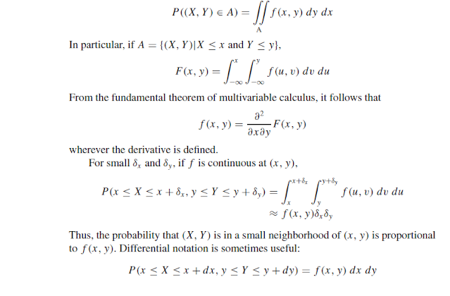
Suppose that $X$ and $Y$ are continuous random variables with a joint cdf, $F(x, y)$. Their joint density function is a piecewise continuous function of two variables, $f (x, y)$. The density function
$f (x, y)$ is nonnegative and $\int_{-\infty}^\infty \int_{-\infty}^\infty f(x,y) dy dx=1$. For any “reasonable” two-dimensional set $A$
For several jointly continuous random variables, we can make the obvious generalizations. The joint density function is a function of several variables, and the marginal density functions are found by integration. There are marginal density functions of various dimensions. Suppose that $X, Y$ , and $Z$ are jointly continuous random variables with density function $f (x, y, z)$. The one-dimensional marginal distribution of $X$ is
Independent Random Variables
Random variables $X1, X2, . . . , Xn$ are said to be independent if their joint cdf factors into the product of their marginal cdf’s:
$F(x1, x2, . . . , xn) = F_{X1} (x1)F_{X2} (x2) · · · F_{Xn} (xn)$
for all $x1, x2, . . . , xn.$
The definition holds for both continuous and discrete random variables. For discrete random variables, it is equivalent to state that their joint frequency function factors; for continuous random variables, it is equivalent to state that their joint density function factors. To see why this is true, consider the case of two jointly continuous random variables, $X$ and $Y$ . If they are independent, then
$F(x, y) = F_X (x)F_Y (y)$
Conditional Distributions


Comments
Post a Comment