Posts

Foundations of Machine Learning CST 312 KTU CS Elective Notes

  Introduction About Me Syllabus What is Machine Learning ( video) Learn the seven steps in Machine Learning ( video) Overview Of Machine Learning Linear Algebra in Machine Learning Module-1 Linear Algebra 1.Geometry of Linear Equations (video) 2.Elimination with Matrices (video) 3.Solving System of equations using Gauss Elimination Method 4.Row Echelon form and Reduced Row Echelon Form 5.Solving system of equations Python code 6. Practice problems Gauss Elimination ( contact) 7.Finding Inverse using Gauss Jordan Elimination (video) 8.Finding Inverse using Gauss Jordan Elimination-Python code 9.Vector spaces and sub spaces 10.Linear Independence 11.Linear Independence, Basis and Dimension (video) 12.Generating set basis and span 13.Rank of a Matrix 14.Linear Mapping and Matrix Representation of Linear Mapping 15.Basis and Change of basis 16. Transformation Matrix in new Basis 17.Image and Kernel 18.Example Problems ( contact) Module 2: Linear Algebra 1.Vector Norms 2.Inner Products 3.

Moment Generating Functions

Image
This section develops and applies some of the properties of the moment-generating function. It turns out, despite its unlikely appearance, to be a very useful tool that can dramatically simplify certain calculations. The moment-generating function (mgf) of a random variable $X$ is  $M(t) =E(e^{t X })$  if the expectation is defined. In the discrete case, $M(t) =\sum_x e^{tx} p(x)$ and in the continuous case, $M(t) =\int_{-\infty}^{\infty}e^{tx} f (x) dx$ The expectation, and hence the moment-generating function, may or may not exist for any particular value of $t$. In the continuous case, the existence of the expectation depends on how rapidly the tails of the density decrease; for example, because the tails of the Cauchy density die down at the rate $x^{−2}$, the expectation does not exist for any $t$ and the moment-generating function is undefined. The tails of the normal density die down at the rate $e^{−x^2}$ , so the integral converges for all $t$. The $r $th moment of a rand

Syllabus Foundations of Machine Learning CST 312 KTU

Syllabus Module 1 (LINEAR ALGEBRA ) Systems of Linear Equations – Matrices, Solving Systems of Linear Equations. Vector Spaces - Linear Independence, Basis and Rank, Linear Mappings. Module 2 (LINEAR ALGEBRA ) Norms - Inner Products, Lengths and Distances, Angles and Orthogonality. Orthonormal Basis, Orthogonal Complement, Orthogonal Projections. Matrix Decompositions - Eigenvalues and Eigenvectors, Eigen decomposition and Diagonalization. Module 3 (PROBABILITY AND DISTRIBUTIONS) Probability Space - Sample Spaces, Probability Measures, Computing Probabilities,Conditional Probability, Baye’s Rule, Independence. Random Variables - Discrete Random Variables (Bernoulli Random Variables, Binomial Distribution, Geometric and Poisson Distribution, Continuous Random Variables (Exponential Density, Gamma Density, Normal Distribution, Beta Density) Module 4 (RANDOM VARIABLES) Functions of a Random Variable. Joint Distributions - Independent Random Variables, Conditional Distributions, Functions

Distributions derived from normal distribution

Image
$χ^2, t,$ and $F$ Distributions we know that the sum of independent gamma random variables that have the same value of $λ$ follows a gamma distribution, and therefore the chi-square distribution with $n$ degrees of freedom is a gamma distribution with $α = n/2$ and $λ = 1/2$ . Its density is From the density function of Proposition A, $f (t) = f (−t)$, so the $t$ distribution is symmetric about zero. As the number of degrees of freedom approaches infinity, the $t$ distribution tends to the standard normal distribution; in fact, for more than 20 or 30 degrees of freedom, the distributions are very close. Figure below shows several $t$ densities. Note that the tails become lighter as the degrees of freedom increase. It can be shown that, for $n > 2, E(W)$ exists and equals $n/(n − 2)$. From the definitions of the $t$ and $F$ distributions, it follows that the square of a $t_n$ random variable follows an $F_{1,n}$ distribution. The Sample Mean and the Sample Variance Let $X_1, . .

Expected Values-Variance,Co Variance and Correlation

Image
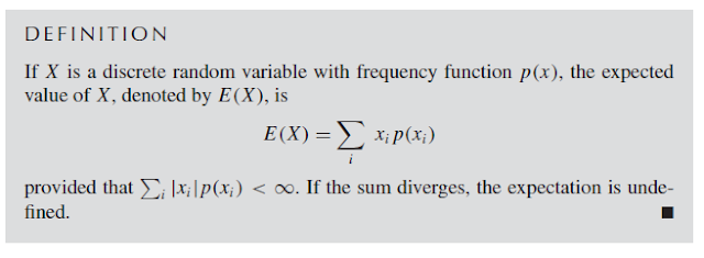
The Expected Value of a Random Variable The concept of the expected value of a random variable parallels the notion of a weighted average. The possible values of the random variable are weighted by their probabilities, as specified in the following definition. $E(X)$ is also referred to as the mean of $X$ and is often denoted by $μ$ or $μX$ . It might be helpful to think of the expected value of $X$ as the center of mass of the frequency function. Imagine placing the masses $p(x_i )$ at the points $x_i$ on a beam; the balance point of the beam is the expected value of  $X$. The definition of expectation for a continuous random variable is a fairly obvious extension of the discrete case—summation is replaced by integration. Expectations of Functions of Random Variables We often need to find E[g(X)], where X is a random variable and g is a fixed function Now suppose that $Y = g(X1, . . . , Xn)$, where $Xi$ have a joint distribution, and that we want to find $E(Y )$. We do not have to fin

Joint Distributions

Image
Joint Distributions concerned with joint probability structure of two or more random variables defined on the same sample space.Joint distributions arise naturally in many applications. • The joint probability distribution of the x, y, and z components of wind velocity can be experimentally measured in studies of atmospheric turbulence. • The joint distribution of the values of various physiological variables in a population of patients is often of interest in medical studies. • A model for the joint distribution of age and length in a population of fish can be used to estimate the age distribution from the length distribution. The age distribution is relevant to the setting of reasonable harvesting policies. The joint behavior of two random variables, $X$ and $Y$, is determined by the cumulative distribution function $F(x, y) = P(X ≤ x, Y ≤ y)$ regardless of whether $X$ and $Y$ are continuous or discrete. The cdf gives the probability that the point $(X, Y )$ belongs to a semi-inf

Random Variables- Discrete and Continuous

Image
Discrete Random Variables A random variable is essentially a random number. As motivation for a definition, let us consider an example. A coin is thrown three times, and the sequence of heads and tails is observed; thus, $\Omega= \{hhh, hht, htt, hth, ttt, tth, thh, tht\}$ Examples of random variables defined on $\Omega$ are (1) the total number of heads, (2) the total number of tails, and (3) the number of heads minus the number of tails. Each of these is a real-valued function defined on $\Omega$; that is, each is a rule that assigns a real number to every point $\omega \in \Omega$ . Since the outcome in $\Omega$ is random, the corresponding number is random as well. In general, a random variable is a function from $\Omega$ to the real numbers. Because the outcome of the experiment with sample space $\Omega$ is random, the number produced by the function is random as well. It is conventional to denote random variables by italic uppercase letters from the end of the alphabet. Fo

Central Limit Theorem

Image
The Law of Large Numbers It is commonly believed that if a fair coin is tossed many times and the proportion of heads is calculated, that proportion will be close to 1/2 . John Kerrich, a South African mathematician, tested this belief empirically while detained as a prisoner during World War II. He tossed a coin 10,000 times and observed 5067 heads. The law of large numbers is a mathematical formulation of this belief. The successive tosses of the coin are modeled as independent random trials. The random variable $X_i$ takes on the value 0 or 1 according to whether the $i$th trial results in a tail or a head, and the proportion of heads in $n$ trials is $\bar{X_n}=\frac{1}{n}\sum_i^n X_i$ The law of large numbers states that $\bar{X_n}$ approaches 1/2 in a sense that is specified by the following theorem. Convergence in Distribution and the Central Limit Theorem In applications, we often want to find $P(a < X < b)$ when we do not know the cdf of $X$ precisely; it is sometimes